Publication-ready moderations with simple slopes in R
Rémi Thériault
February 8, 2022
Source:vignettes/moderation.Rmd
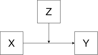
moderation.RmdSometimes in research, we want to know whether the effect of variable X on Y is affected by a third variable, variable Z. In other terms, we ask if there is an interaction between variables X and Z, and their effects on Z.
Note that this is different from mediation, where the mediator is the mechanism that explains the link between X and Y (rather than a variable that modifies an existing relationship like in moderation).

In R, we conduct moderation analyses using straight
linear models with the lm function, and we specify
interaction effects with the * operator. Not everyone is familiar with
using lm however, so rempsyc provides a
(relatively) simpler interface where it is straightforward what variable
is the moderator, and which one is the predictor. Although it does not
make a difference between the lm model, for some (e.g.,
that find the lm function scary), it can be helpful to
think about these variables in this way. The other benefit is that it
provides a useful effect size and its 95% confidence interval, and
formats everything in a table ready to be exported to word through
nice_table.
The topic of moderations and simple slopes can be a complex one. It is not the goal of this tutorial to describe the theory behind it, only to show a practical way to do them. For a more detailed reading on the topic, please see one of the existing excellent sources on the topic (1, 2, 3).
Getting started
Let’s first load the demo data. This data set comes with base
R (meaning you have it too and can directly type this
command into your R console).
head(mtcars)## mpg cyl disp hp drat wt qsec vs am gear carb
## Mazda RX4 21.0 6 160 110 3.90 2.620 16.46 0 1 4 4
## Mazda RX4 Wag 21.0 6 160 110 3.90 2.875 17.02 0 1 4 4
## Datsun 710 22.8 4 108 93 3.85 2.320 18.61 1 1 4 1
## Hornet 4 Drive 21.4 6 258 110 3.08 3.215 19.44 1 0 3 1
## Hornet Sportabout 18.7 8 360 175 3.15 3.440 17.02 0 0 3 2
## Valiant 18.1 6 225 105 2.76 3.460 20.22 1 0 3 1Load the rempsyc package:
Note: If you haven’t installed this package yet, you will need to install it via the following command:
install.packages("rempsyc"). Furthermore, you may be asked to install the following packages if you haven’t installed them already (you may decide to install them all now to avoid interrupting your workflow if you wish to follow this tutorial from beginning to end):
pkgs <- c("effectsize", "flextable", "interactions")
install_if_not_installed(pkgs)
For moderations and simple slopes, we usually want to standardize (or at least center) our variables.
mtcars2 <- lapply(mtcars, scale) |> as.data.frame()Simple moderation: nice_mod
moderations <- nice_mod(
  data = mtcars2,
  response = "mpg",
  predictor = "gear",
  moderator = "wt"
)
moderations
## Dependent Variable Predictor df B t p
## 1 mpg gear 28 -0.08718042 -0.7982999 4.314156e-01
## 2 mpg wt 28 -0.94959988 -8.6037724 2.383144e-09
## 3 mpg gear:wt 28 -0.23559962 -2.1551077 3.989970e-02
## sr2 CI_lower CI_upper
## 1 0.004805465 0.0000000000 0.02702141
## 2 0.558188818 0.3142326391 0.80214500
## 3 0.035022025 0.0003502202 0.09723370If we want it to look nice
(my_table <- nice_table(moderations, highlight = TRUE))Dependent Variable |
Predictor |
df |
b* |
t |
p |
sr2 |
95% CI |
|---|---|---|---|---|---|---|---|
mpg |
gear |
28 |
-0.09 |
-0.80 |
.431 |
.00 |
[0.00, 0.03] |
wt |
28 |
-0.95 |
-8.60 |
< .001*** |
.56 |
[0.31, 0.80] |
|
gear × wt |
28 |
-0.24 |
-2.16 |
.040* |
.04 |
[0.00, 0.10] |
Note: The sr2 (semi-partial correlation squared, also known as delta R-square) allows us to quantify the unique contribution (proportion of variance explained) of an independent variable on the dependent variable, over and above the other variables in the model. sr2 is often considered a better indicator of the practical relevance of a variable.
Open (or save) table to Word
Let’s save it to word for use in a publication (optional).
# Open in Word
print(my_table, preview = "docx")

# Save in Word
flextable::save_as_docx(my_table, path = "moderations.docx")
Simple slopes: nice_slopes
You might have heard about “simple slopes” before. But what does that mean? Essentially, this means looking at the strength (regression coefficient) and significance of the slope, when subsetting for observations that are high, low, or average on a variable, typically the moderating variable. A bit further down, this will get clearer by looking at the plot of the interaction, which shows one slope for observations that are high on the wt (moderating) variable, a second slope for those that are low, and a third slope for those that are average.
Let’s extract the simple slopes now, including the sr2.
slopes <- nice_slopes(
  data = mtcars2,
  response = "mpg",
  predictor = "gear",
  moderator = "wt"
)
slopes
## Dependent Variable Predictor (+/-1 SD) df B t p
## 1 mpg gear (LOW-wt) 28 0.14841920 1.0767040 0.29080233
## 2 mpg gear (MEAN-wt) 28 -0.08718042 -0.7982999 0.43141565
## 3 mpg gear (HIGH-wt) 28 -0.32278004 -1.9035367 0.06729622
## sr2 CI_lower CI_upper
## 1 0.008741702 0 0.03886052
## 2 0.004805465 0 0.02702141
## 3 0.027322839 0 0.08179662
nice_table(slopes, highlight = TRUE)Dependent Variable |
Predictor (+/-1 SD) |
df |
b* |
t |
p |
sr2 |
95% CI |
|---|---|---|---|---|---|---|---|
mpg |
gear (LOW-wt) |
28 |
0.15 |
1.08 |
.291 |
.01 |
[0.00, 0.04] |
gear (MEAN-wt) |
28 |
-0.09 |
-0.80 |
.431 |
.00 |
[0.00, 0.03] |
|
gear (HIGH-wt) |
28 |
-0.32 |
-1.90 |
.067 |
.03 |
[0.00, 0.08] |
In this specific case, the interaction is significant but none of the simple slopes. This means that although the two slopes are significantly different from each other, taken individually, the slopes aren’t significantly different from a straight line.
The neat thing is that you can add as many dependent variables at once as you want.
# Moderations
nice_mod(
  data = mtcars2,
  response = c("mpg", "disp", "hp"),
  predictor = "gear",
  moderator = "wt"
) |>
  nice_table(highlight = TRUE)
Dependent Variable |
Predictor |
df |
b* |
t |
p |
sr2 |
95% CI |
|---|---|---|---|---|---|---|---|
mpg |
gear |
28 |
-0.09 |
-0.80 |
.431 |
.00 |
[0.00, 0.03] |
wt |
28 |
-0.95 |
-8.60 |
< .001*** |
.56 |
[0.31, 0.80] |
|
gear × wt |
28 |
-0.24 |
-2.16 |
.040* |
.04 |
[0.00, 0.10] |
|
disp |
gear |
28 |
-0.07 |
-0.70 |
.492 |
.00 |
[0.00, 0.02] |
wt |
28 |
0.83 |
7.67 |
< .001*** |
.43 |
[0.19, 0.67] |
|
gear × wt |
28 |
-0.09 |
-0.81 |
.422 |
.00 |
[0.00, 0.03] |
|
hp |
gear |
28 |
0.42 |
2.65 |
.013* |
.11 |
[0.00, 0.27] |
wt |
28 |
0.93 |
5.75 |
< .001*** |
.53 |
[0.29, 0.77] |
|
gear × wt |
28 |
0.15 |
0.96 |
.346 |
.01 |
[0.00, 0.07] |
# Simple slopes
nice_slopes(
  data = mtcars2,
  response = c("mpg", "disp", "hp"),
  predictor = "gear",
  moderator = "wt"
) |>
  nice_table(highlight = TRUE)
Dependent Variable |
Predictor (+/-1 SD) |
df |
b* |
t |
p |
sr2 |
95% CI |
|---|---|---|---|---|---|---|---|
mpg |
gear (LOW-wt) |
28 |
0.15 |
1.08 |
.291 |
.01 |
[0.00, 0.04] |
gear (MEAN-wt) |
28 |
-0.09 |
-0.80 |
.431 |
.00 |
[0.00, 0.03] |
|
gear (HIGH-wt) |
28 |
-0.32 |
-1.90 |
.067 |
.03 |
[0.00, 0.08] |
|
disp |
gear (LOW-wt) |
28 |
0.01 |
0.09 |
.926 |
.00 |
[0.00, 0.00] |
gear (MEAN-wt) |
28 |
-0.07 |
-0.70 |
.492 |
.00 |
[0.00, 0.02] |
|
gear (HIGH-wt) |
28 |
-0.16 |
-0.97 |
.339 |
.01 |
[0.00, 0.03] |
|
hp |
gear (LOW-wt) |
28 |
0.27 |
1.34 |
.190 |
.03 |
[0.00, 0.11] |
gear (MEAN-wt) |
28 |
0.42 |
2.65 |
.013* |
.11 |
[0.00, 0.27] |
|
gear (HIGH-wt) |
28 |
0.58 |
2.33 |
.027* |
.09 |
[0.00, 0.22] |
Pro tip: Both the
nice_mod()andnice_slopes()functions take the same argument, so you can just copy-paste the first and change the function call to save time!
Special cases
Covariates
You can also have more complicated models, like with added covariates.
Moderations
nice_mod(
  data = mtcars2,
  response = "mpg",
  predictor = "gear",
  moderator = "wt",
  covariates = c("am", "vs")
) |>
  nice_table(highlight = TRUE)
Dependent Variable |
Predictor |
df |
b* |
t |
p |
sr2 |
95% CI |
|---|---|---|---|---|---|---|---|
mpg |
gear |
26 |
-0.11 |
-0.88 |
.388 |
.00 |
[0.00, 0.02] |
wt |
26 |
-0.70 |
-5.07 |
< .001*** |
.15 |
[0.02, 0.28] |
|
am |
26 |
0.13 |
0.86 |
.399 |
.00 |
[0.00, 0.02] |
|
vs |
26 |
0.32 |
3.24 |
.003** |
.06 |
[0.00, 0.14] |
|
gear × wt |
26 |
-0.25 |
-2.56 |
.017* |
.04 |
[0.00, 0.09] |
Simple slopes
nice_slopes(
  data = mtcars2,
  response = "mpg",
  predictor = "gear",
  moderator = "wt",
  covariates = c("am", "vs")
) |>
  nice_table(highlight = TRUE)
Dependent Variable |
Predictor (+/-1 SD) |
df |
b* |
t |
p |
sr2 |
95% CI |
|---|---|---|---|---|---|---|---|
mpg |
gear (LOW-wt) |
26 |
0.14 |
0.89 |
.383 |
.00 |
[0.00, 0.02] |
gear (MEAN-wt) |
26 |
-0.11 |
-0.88 |
.388 |
.00 |
[0.00, 0.02] |
|
gear (HIGH-wt) |
26 |
-0.36 |
-2.25 |
.033* |
.03 |
[0.00, 0.08] |
In this case, only the third row is significant, which means that
those who are high on the wt variable (above one standard
deviation) have significantly lower mpg the higher their
gear. We can plot this in the more traditional way:
# First need to define model for plot function
mod <- lm(mpg ~ gear * wt + am + vs, data = mtcars2)

# Plot the model
library(interactions)
interact_plot(mod, pred = "gear", modx = "wt", interval = TRUE)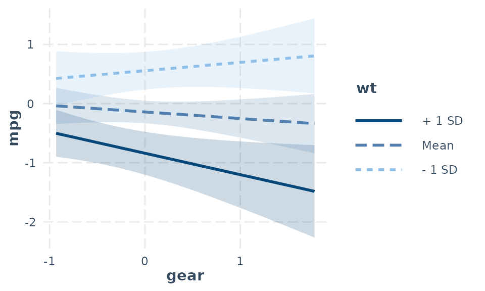
Note: If you haven’t installed this package yet, you will need to install it via the following command:
install.packages(interactions). Furthermore, know that this plot can be heavily customized with available arguments for publication purposes, but I won’t be going into these details here.
Three-way interaction
Let’s make a three-way interaction for example.
Note that for the simple slopes, for now, the second moderator needs to be a dichotomic variable (and the first moderator a continuous variable). We’ll reset the am variable for this purpose for now.
mtcars2$am <- mtcars$amModerations
nice_mod(
  response = "mpg",
  predictor = "gear",
  moderator = "disp",
  moderator2 = "am",
  data = mtcars2
) |>
  nice_table(highlight = TRUE)
Dependent Variable |
Predictor |
df |
b* |
t |
p |
sr2 |
95% CI |
|---|---|---|---|---|---|---|---|
mpg |
gear |
24 |
-0.43 |
-0.68 |
.500 |
.00 |
[0.00, 0.02] |
disp |
24 |
-3.04 |
-3.16 |
.004** |
.06 |
[0.00, 0.14] |
|
am |
24 |
-0.21 |
-0.35 |
.731 |
.00 |
[0.00, 0.01] |
|
gear × disp |
24 |
-1.09 |
-1.09 |
.287 |
.01 |
[0.00, 0.03] |
|
gear × am |
24 |
1.34 |
2.41 |
.024* |
.04 |
[0.00, 0.09] |
|
disp × am |
24 |
-0.07 |
-0.08 |
.936 |
.00 |
[0.00, 0.00] |
|
gear × disp × am |
24 |
1.90 |
2.21 |
.037* |
.03 |
[0.00, 0.08] |
Simple slopes
nice_slopes(
  data = mtcars2,
  response = "mpg",
  predictor = "gear",
  moderator = "disp",
  moderator2 = "am"
) |>
  nice_table(highlight = TRUE)
Dependent Variable |
am |
Predictor (+/-1 SD) |
df |
b* |
t |
p |
sr2 |
95% CI |
|---|---|---|---|---|---|---|---|---|
mpg |
0.00 |
gear (LOW-disp) |
24 |
1.11 |
1.57 |
.131 |
.02 |
[0.00, 0.05] |
0.00 |
gear (MEAN-disp) |
24 |
-1.53 |
-1.49 |
.148 |
.01 |
[0.00, 0.05] |
|
0.00 |
gear (HIGH-disp) |
24 |
-4.16 |
-1.56 |
.131 |
.02 |
[0.00, 0.05] |
|
1.00 |
gear (LOW-disp) |
24 |
-0.00 |
-0.01 |
.990 |
.00 |
[0.00, 0.00] |
|
1.00 |
gear (MEAN-disp) |
24 |
1.17 |
2.59 |
.016* |
.04 |
[0.00, 0.10] |
|
1.00 |
gear (HIGH-disp) |
24 |
2.34 |
2.71 |
.012* |
.05 |
[0.00, 0.11] |
Complex models: nice_lm
For more complicated models not supported by nice_mod,
one can define the model in the traditional way and feed it to
nice_lm and nice_lm_slopes instead. They
support multiple lm models as well.
nice_lm
model1 <- lm(mpg ~ cyl + wt * hp, mtcars2)
model2 <- lm(qsec ~ disp + drat * carb, mtcars2)
my.models <- list(model1, model2)
nice_lm(my.models) |>
  nice_table(highlight = TRUE)
Dependent Variable |
Predictor |
df |
b |
t |
p |
sr2 |
95% CI |
|---|---|---|---|---|---|---|---|
mpg |
cyl |
27 |
-0.11 |
-0.72 |
.479 |
.00 |
[0.00, 0.01] |
wt |
27 |
-0.62 |
-5.70 |
< .001*** |
.14 |
[0.02, 0.25] |
|
hp |
27 |
-0.29 |
-2.40 |
.023* |
.02 |
[0.00, 0.06] |
|
wt × hp |
27 |
0.29 |
3.23 |
.003** |
.04 |
[0.00, 0.10] |
|
qsec |
disp |
27 |
-0.43 |
-1.97 |
.059 |
.07 |
[0.00, 0.20] |
drat |
27 |
-0.33 |
-1.53 |
.138 |
.04 |
[0.00, 0.14] |
|
carb |
27 |
-0.51 |
-3.32 |
.003** |
.20 |
[0.00, 0.41] |
|
drat × carb |
27 |
-0.23 |
-1.08 |
.289 |
.02 |
[0.00, 0.09] |
The same applies to simple slopes, this time we use the
nice_lm_slopes function. It supports multiple
lm models as well, but the predictor and moderator need to
be the same for these models (the dependent variable can change).
nice_lm_slopes
model1 <- lm(mpg ~ gear * wt, mtcars2)
model2 <- lm(disp ~ gear * wt, mtcars2)
my.models <- list(model1, model2)
nice_lm_slopes(my.models, predictor = "gear", moderator = "wt") |>
  nice_table(highlight = TRUE)
Dependent Variable |
Predictor (+/-1 SD) |
df |
b |
t |
p |
sr2 |
95% CI |
|---|---|---|---|---|---|---|---|
mpg |
gear (LOW-wt) |
28 |
0.15 |
1.08 |
.291 |
.01 |
[0.00, 0.04] |
gear (MEAN-wt) |
28 |
-0.09 |
-0.80 |
.431 |
.00 |
[0.00, 0.03] |
|
gear (HIGH-wt) |
28 |
-0.32 |
-1.90 |
.067 |
.03 |
[0.00, 0.08] |
|
disp |
gear (LOW-wt) |
28 |
0.01 |
0.09 |
.926 |
.00 |
[0.00, 0.00] |
gear (MEAN-wt) |
28 |
-0.07 |
-0.70 |
.492 |
.00 |
[0.00, 0.02] |
|
gear (HIGH-wt) |
28 |
-0.16 |
-0.97 |
.339 |
.01 |
[0.00, 0.03] |
Thanks for checking in
Make sure to check out this page again if you use the code after a time or if you encounter errors, as I periodically update or improve the code. Feel free to contact me for comments, questions, or requests to improve this function at https://github.com/rempsyc/rempsyc/issues. See all tutorials here: https://remi-theriault.com/tutorials.